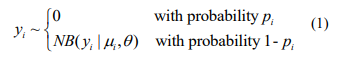
ОТРИЦАТЕЛЬНАЯ БИНОМИАЛЬНАЯ РЕГРЕССИЯ С НУЛЕВЫМ РАЗДУВОМ ДЛЯ ОЦЕНКИ ОТНОСИТЕЛЬНОГО СОДЕРЖАНИЯ В МИКРОБИОМНЫХ ИССЛЕДОВАНИЯХ

ZERO-INFLATED NEGATIVE BINOMIAL REGRESSION FOR DIFFERENTIAL ABUNDANCE TESTING IN MICROBIOME STUDIES
Conflict of Interest
None declared.
Xinyan Zhang1, Himel Mallick2, Nengjun Yi1*
1Department of Biostatistics, University of Alabama at Birmingham, Birmingham, AL 35294, USA, 2 Department of Biostatistics, Harvard T.H. Chan School of Public Health, Boston, MA 02115, USA; Program in Medical and Population Genetics, The Broad Institute, Cambridge, MA 02142, USA, 3Department of Biostatistics, University of Alabama at Birmingham, Birmingham, AL 35294, USA 1,2Joint First Authors
*To whom correspondence should be addressed.
Associate editor: Giancarlo Castellano
Received on 03 November 2016, revised on 01 December 2016, accepted on 12 December 2016.
Abstract
Motivation: The human microbiome plays an important role in human health and disease. The composition of the human microbiome is influenced by multiple factors and understanding these factors is critical to elucidate the role of the microbiome in health and disease and for development of new diagnostics or therapeutic targets based on the microbiome. 16S ribosomal RNA (rRNA) gene targeted amplicon sequencing is a commonly used approach to determine the taxonomic composition of the bacterial community. Operational taxonomic units (OTUs) are clustered based on generated sequence reads and used to determine whether and how the abundance of microbiome is correlated with some characteristics of the samples, such as health/disease status, smoking status, or dietary habit. However, OTU count data is not only overdispersed but also contains an excess number of zero counts due to undersampling. Efficient analytical tools are therefore needed for downstream statistical analysis which can simultaneously account for overdispersion and sparsity in microbiome data.
Results: In this paper, we propose a Zero-inflated Negative Binomial (ZINB) regression for identifying differentially abundant taxa between two or more populations. The proposed method utilizes an Expectation Maximization (EM) algorithm, by incorporating a two-part mixture model consisting of (i) a negative binomial model to account for overdispersion and (ii) a logistic regression model to account for excessive zero counts. Extensive simulation studies are conducted which indicate that ZINB demonstrates better performance as compared to several state-of-the-art approaches, as measured by the area under the curve (AUC). Application to two real datasets indicate that the proposed method is capable of detecting biologically meaningful taxa, consistent with previous studies.
Availability: The software implementation of ZINB is available at: http://www.ssg.uab.edu/bhglm/.
Supplementary information: Supplementary data are available at Journal of Bioinformatics and Genomics online.
Keywords: Differential Abundance Testing, EM Algorithm, Human Microbiome, Metagenomics, OTU, Zero-inflated Negative Binomial.
Contact: nyi@uab.edu
1. Introduction
The advent of next-generation sequencing (NGS) technology enables the generation of large volume of metagenomic sequencing data (Gilbert, Meyer, & Bailey, 2011). This opens a new era of genomics study to explore microbial communities sampled directly from environments without isolation and cultivation (Cho & Blaser, 2012; Hugenholtz, 2002; Wooley & Ye, 2009). One of the environment is human or mammalian body which harbors a dense microbial population across different body sites, containing taxa across the tree of life including bacteria, viruses, micro-eukaryotes, and archaea (Dethlefsen, McFall-Ngai, & Relman, 2007; Whitman, Coleman, & Wiebe, 1998). The combination of microbiota, their genomes (metagenome), and the host environment forms human or mammalian microbiome (Cho & Blaser, 2012). An important research interest in human microbiome study is to assess whether and how two or more microbiome communities differ from each other. Many factors can influence the human microbiome composition (Turnbaugh et al., 2007). These factors include the host genotype (Spor, Koren, & Ley, 2011), host physiological status such as aging (Biagi et al., 2010), host pathophysiological status (Turnbaugh et al., 2009), host lifestyle such as dietary habit (De Filippo et al., 2010; Wu et al., 2011), and host environment (DominguezBello et al., 2010). Different studies have investigated the association between the human microbiome and human diseases such as obesity (Turnbaugh et al., 2006), diabetes (Samuel & Gordon, 2006), inflammatory bowel disease (IBD) (Frank et al., 2007), and cancers (Holmes, Li, Athanasiou, Ashrafian, & Nicholson, 2011). The findings from these studies demonstrated that the human microbiome has extraordinary potential implications in new therapeutic targets or biomarkers for disease prevention and early diagnosis (Collison et al., 2012; Knights, Parfrey, Zaneveld, Lozupone, & Knight, 2011; Segata et al., 2011; Virgin & Todd, 2011). 16S ribosomal RNA (rRNA) gene targeted amplicon sequencing is a commonly used approach to determine the taxonomic composition and species diversity of the bacterial community (Matsen, Kodner, & Armbrust, 2010). Hypervariable regions within the gene are amplified and sequenced, and sequence reads are clustered into operational taxonomic units (OTUs) based on sequence similarity (Ghodsi, Liu, & Pop, 2011). Representative sequences from each cluster are then classified taxonomically by alignment against a database of previously characterized 16S ribosomal DNA (rDNA) reference sequences. The resulting OTU counts are then used to determine whether and how the abundance of microbiome is correlated with some characteristics of the samples, such as health/disease status, smoking status, or dietary habit.
However, the OTU/taxa data are high-dimensional with added complexity leading to several statistical challenges. The first challenge of microbiome data is how to properly account for variability induced by differences in sequencing depth across samples. This is due to our inability to accurately specify the exact number of sequences to be measured on a sample using currently available technology. Although the total number of sequences for a given sample is not associated with any biological feature of the sample, it affects the OTU counts, and hence, should be accounted for in downstream bioinformatic and statistical analysis. A common approach to account for this variation in the total number of sequences is the total-sum scaling (TSS) normalization, i.e. conversion of the sequence counts to relative abundance (i.e., taxon counts/total counts) within a particular sample (Wagner, Robertson, & Harris, 2011). However, using total counts as the normalization/scaling factor may be problematic and may lead to biases in differential abundance estimates (Knights et al., 2011; Kostic et al., 2012; Paulson, Stine, Bravo, & Pop, 2013). To adjust for differential sequencing depths, different approaches such as cumulative sum scaling (CSS) (Paulson et al., 2013), trimmed mean of M-values (TMM) (Robinson & Oshlack, 2010), and relative log expression (RLE) (Anders & Huber, 2010), have been proposed in the literature. Furthermore, due to the association between detected number of features (OTUs) and the depth of coverage in different samples, only a few OTUs are shared in various samples, whereas the rest are only present in a small proportion of samples, resulting in excess of zero counts in the OTUs count matrix (Paulson et al., 2013; Peng, Li, & Liu, 2015).
Second, OTU counts are over-dispersed, meaning the variance of the counts varies with the value of the mean. For such overdispersed count data, standard methods such as Poisson regression can result in high false positives (Peng et al., 2015; White, Nagarajan, & Pop, 2009). The overdispersed data have been widely studied in differential expression analysis in microarray and high-throughput sequencing (serial analysis of gene expression (SAGE) (Velculescu, Zhang, Vogelstein, & Kinzler, 1995) and RNA-seq) (McMurdie & Holmes, 2014). Differential abundance analysis in microbiome is a direct analogy to differential expression analysis. Many analytical tools (edgeR and DESeq) developed for differential expression analysis of RNA-Seq data can be adapted to differential abundance analysis of OTUs (Anders & Huber, 2010; Robinson, McCarthy, & Smyth, 2010). For example, White et al. (2009) extended the methods in differential expression analysis to microbiome studies by converting the raw abundances to proportions, which represent the relative contribution of each feature for each individual. This method was implemented in the software Metastats. However, microbiome data have the distinct characteristic of zeroinflation, which is notably less severe in RNA-seq data. To this end, various zero-inflated models have been proposed to correct for sparse counts in microbiome measurements. Paulson et al. (2013) proposed a zero-inflated Gaussian mixture model for modeling the CSS-normalized logtransformed count data using an Expectation Maximization (EM) algorithm, implemented in the Bioconductor package metagenomeSeq. Sohn et al. (2015) implemented a ratio approach for identifying differential abundance (RAIDA) by utilizing the ratio between features in a modified zero-inflated lognormal model. Peng et al. (2015) proposed a zero-inflated beta regression (ZIBSeq) approach for modeling the TSSnormalized relative abundance data. All these zero-inflated methods are designed to analyze microbiome data after a suitable normalization and/or transformation. However, differential abundance estimates based on these methods may not be interpretable on the original scale, leading to challenges in future prediction tasks and replication studies.
To address the above limitations, we propose a Zero-inflated Negative Binomial (ZINB) mixture model, which directly models the raw OTU counts. We implemented our model in R package BhGLM by utilizing an EM algorithm incorporating a two-part mixture model consisting of (i) negative binomial model to account for over-dispersion and (ii) a logistic regression model to account for zero-inflation. In our simulations, we show that ZINB outperforms DESeq, edgeR, and metagenomeSeq in various sparse scenarios in terms of Area under the Curve (AUC) estimates. Application to two real microbiome data sets reveal biologically significant taxa, which are consistent with previous studies. The software implementation of ZINB is freely available at: http://www.ssg.uab.edu/bhglm/.
2. Methods
Assume that there are n samples and m features. In 16S rRNA microbiome data, the features refer to OTUs, species, or genus, etc. Let Cij be the observed count for i-th sample and jth feature, and Ti be the total read for i-th sample (also referred to as depths of coverage or library size) or a linear scaling factor that accounts for its library size. Let Xi be a factor indicating host health/disease status, physiological status such as aging, or lifestyle such as dietary habit, etc. In differential abundance analysis, the goal is to determine differentially abundant microbial features between groups defined by the host factor. We directly model the raw count data with the zeroinflated negative binomial model. To adjust for differential sequencing depth, the natural logarithm of total counts (per sample) are included as offset in the negative binomial model. This allows us to handle the raw data matrix without normalization, leading to interpretable differential abundance estimates. In the following subsection, we describe our model and algorithm.
2.1. Zero-inflated Negative Binomial (ZINB) Model
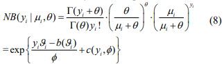
ZINB models assume that observed zero counts may come from either a degenerate distribution having the point mass at zero or a negative binomial distribution and observed non-zero counts come exclusively from the negative binomial distribution. Therefore, the count response for feature j, i.e., yi = Cij, follows the mixture distribution:
where  and
and  are the mean and the shape parameter of the negative binomial distribution
  , respectively, and pi are the mixture probability parameters. The mean parameters are related to the variables Xi (including the intercept) via the link function logarithm:

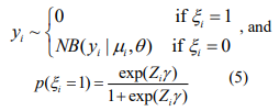
where  is the offset, which corrects for the variation of the library size. The mixture probability parameters are modeled by the logistic regression:
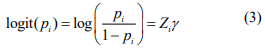
where Zi includes variables that are potentially associated with the zero state. We can include only intercept in Zi (as in the simulation study and real data analysis). However, our method can be applied to general cases.
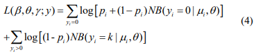
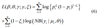
The log-likelihood function for the parameters (β, θ) and γ is given by
The first term in the log-likelihood includes both (β, θ) and γ and thus complicates the maximization of the log-likelihood. In principle, this likelihood can be optimized directly by the Newton-Raphson algorithm (as implemented by the zeroinfl function in the R package pscl). However, the NewtonRaphson algorithm for fitting this model is known to be unstable and have severe non-convergence issues in small samples (Mallick & Tiwari, 2016). We thus propose an EM algorithm, which is stable and efficient, leading to accurate estimation and inference.
2.2. EM algorithm for fitting the ZINB model
The EM algorithm introduces a vector of latent indictor variables  to distinguish the zero state from the negative binomial state, where ξi = 1 when yi is from the zero state, and ξi = 0 when yi is from the negative binomial state. With the indicator variables, the ZINB model can be expressed as
The log-likelihood with the complete data (y, ξ) is given by
The EM algorithm replaces the indictor variables {ξ i} by their conditional expectations {ξ i} (E-step), and then updates the coefficients β and γ and the shape parameter  by maximizing
  (M-step). When the EM algorithm converges, we obtain the estimate
  that maximizes the log-likelihood
  . In the E-step, we calculate the conditional expectations of the indictor variables {ξi}. The conditional expectation of ξi can be easily calculated as:
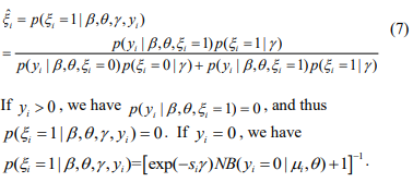
In the M-step, we update the parameters  by maximizing
  . The coefficients β and γ can be separately updated, because γ is only involved in the first term of the log-likelihood,
  , and β and θ are only involved in the second term
 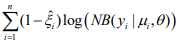 . The first term is the log-likelihood for an unweighted binomial regression of
  on S, and the second term is the loglikelihood for a weighted negative binomial regression of y on X with the weights
  . The parameters β and θ can be updated by fitting the weighted negative binomial regression, and γ can be updated by fitting the unweighted binomial regression.
At convergence of the algorithm, we summarize the inferences using the latest estimate  and its covariance
  , which can be obtained from the final weighted negative binomial model. Thus, we can get the maximum likelihood estimates of the coefficients βj, which stands for the parameter coefficient for jth predictor, and their confidence intervals, and test the hypothesis H0: βj = 0 by using the statistic
  , which approximately follow the standard normal distribution.
2.3. IWLS algorithm for fitting the negative binomial model
The above EM algorithm needs fitting a weighted negative binomial model. We extend the IWLS (Iterative Weighted Least Square) algorithm for generalized linear models to fit the weighted negative binomial model. Our algorithm is based on the well-known fact that given the shape parameter  the negative binomial density has the exponential form:
where 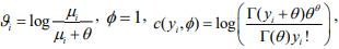 and
and  . Therefore, the negative binomial model is a special case of generalized linear models (GLMs) for any fixed .
The IWLS algorithm for fitting the negative binomial model proceeds as follows. Given the shape parameter , the estimate of  can be obtained by fitting the weighted normal linear model:
where  . The pseudo-response
  and pseudo-weights wi are calculated by
where 
 ,
,  and
and  and
and  are the current estimates of β and θ, respectively. Conditional on β, the shape parameter θ can be updated by maximizing the NB likelihood using the standard Newton-Raphson algorithm.
3. Results
3.1. Simulation Studies
We performed extensive simulations to benchmark our method as compared to several state-of-the art approaches including DESeq, edgeR, and metagenomeSeq. To simulate count data for each feature, we generated OTU counts, cij, from the zero-inflated negative binomial distribution defined in (1). The ranges of the parameters in the simulation studies are described below.
We simulated OTU-level count data with 1000 features for n samples in each of two groups. The sample size n in each group was set to be 50, 100, and 150. The effects of the first 50 features were set to be non-zero, and the others had zero effects. In this setting, the parameter Ti denotes the scaling factor for sample i. We randomly set the offset log(Ti) from the range [0.1, 3.5], the coefficient  from three values (0.5, 1.0, 1.5), and the shape parameter
  from the range [0.1, 8]. To simulate excess amount of zeros for each feature, we randomly generated from a Bernoulli trial with a preset proportion of zeros. We tested five proportions of zeros by varying pi = (0.1, 0.2, 0.3, 0.4, 0.5). We set these ranges of the parameters similar to those in Sohn et al. (2015). The ranges of all the parameters used in the simulation are summarized in Table 1.
Table 1 - Summary of Parameter Ranges in Simulation Studies
| Parameter | Ranges |
| Logarithm of Scaling Factor log(Ti) | Unifrom [0.1, 3.5] |
| Shape Parameter |
Uniform [0.1, 8] |
| Coefficient Estimate |
(0.5, 1.0, 1.5) |
| Proportion pi | (0.1, 0.2, 0.3, 0.4, 0.5) |
We carried out differential abundance analysis for each simulated feature by using the following methods:
1. edgeR – exactTest - an exact binomial test with negative binomial model preceded by TMM normalization (Robinson et al., 2010).
2. DESeq – nbinomTest – a negative binomial conditioned test similar to edgeR but preceding RLE normalization (Anders & Huber, 2010)..
3. metagenomeSeq – fitZig and fitFeatureModel. An Expectation-Maximization estimate of the posterior probabilities of differential abundance based on a zero inflated Gaussian model and zero-inflated log-normal mixture model respectively preceding a CSS normalization and log-transformation (Paulson et al., 2013).
4. BhGLM – Zero-inflated Negative Binomial model using Expectation-Maximization for each feature without any normalization.
For each combination of parameters, the procedure was repeated 100 times. All tests were corrected for multiple testing using Benjamini-Hochberg method to control the False Discovery Rate at the alpha level of 0.05. AUC, power, and false positive rate were calculated to compare the performance of each method. The simulations and real data analyses rely on the following R packages: BhGLM, DESeq, edgeR, foreach, ggplot2, metagenomSeq, phyloseq, reshape2, and ROCR. The reproducible simulation code in R is available upon request from the first authors.
Curves comparing AUC, power, and type I error rates are shown in Figures 1-3 to illustrate the performance of BhGLMZINB, DESeq, edgeR, and metagenomeSeq (fitZig and fitFeatureModel) on synthetic data with different proportions of zeros in detecting significant differentially abundant features for three different sample sizes n = 100, 200, and 300 respectively. Corresponding AUC, power, and type I error quantities are also listed in Tables A.1-A.3 (see Appendix).
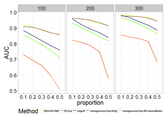
Fig. 1 - Comparison of AUC for Different Methods with Different Zero Proportions and Sample Sizes
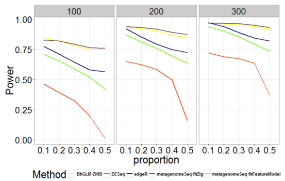
Fig. 2 - Comparison of Power for Different Methods with Different Zero Proportions and Sample Sizes
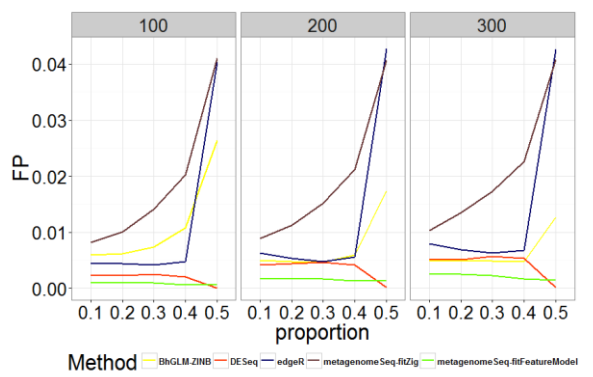
Fig. 3 - Comparison of Type I Error Rates for Different Methods with Different Zero Proportions and Sample Sizes
As shown in Figures 1-2 and Tables A.1-A.2, zero-inflated methods (BhGLM-ZINB, and metagenomeSeq-fitZig) performed similarly on simulated zero inflated data with respect to AUC. When the sample size is low (n=100) and the zero-inflation is 50%, the AUCs of BhGLM-ZINB and metagenomeSeq-fitZig are 0.862 and 0.858, respectively. With the same sample size but 10% zero-inflation, the AUCs of BhGLM-ZINB, and metagenomeSeq-fitZig were 0.921 and 0.910, respectively. With respect to empirical power, metagenomeSeq-fitZig performs slightly well than BhGLMZINB for ≥30% zero-inflation, while BhGLM-ZINB performs slightly better than metagenomeSeq-fitZig when the zeroinflation is 10%. On the other hand, other three methods, DESeq, edgeR, and metagenomeSeq-fitFeatureModel, have much lower power regardless of the sparsity level. As the proportion of zeroes increases, the empirical power of these methods worsens considerably. In terms of Type-I error rates, BhGLM-ZINB performs consistently better than metagenomeSeq-fitFeatureModel across all zero proportions. When the amount of zero-inflation is 50% and n = 100, BhGLM-ZINB controls the type I error rate at 0.026, while metagenomeSeq-fitFeatureModel and edgeR both have a much higher type I error rate (0.041 and 0.040 respectively). In all scenarios, the type I error rates are higher for DESeq, edgeR, and metagenomeSeq-fitFeatureModel, whereas for the proposed method, it is well-controlled, always lower than 0.03. In summary, our simulation indicates that the proposed ZINB method is consistently high in power along with wellcontrolled type I error.
3.2. Real Data Analysis
3.2.1. Lung Microbiome Data
We applied our method to a lung microbiome data from Charlson et al. (2011). The data was sampled in the respiratory flora from six healthy individuals. Among them, three individuals were smokers and the other three were nonsmokers. The two-bronchoscope procedure was used to sample the respiratory tract, followed by a serial bronchoalveolar lavage and lower-airway protected brushes. A more detailed description of the lung microbiome samples, collection, and protocols is available in Charlson et al. (2011). The processed OTU level data was acquired directly from the R package metagenomeSeq. After the rare features were trimmed, we only include 259 features in our analysis. Differential abundance analysis to determine the associations between the remaining features with smoking status of 66 samples was carried out.
Among them, we have listed the top ten significant taxa in Figure 4. Some of the features are consistent with the significant taxa selected by the method metagenomeSeq-fitZig. The first three taxa are Neisseria polysaccharea, Neisseria meningitides, and Neisseria elongate. Neisseria meningitides has been reported as an uncommon cause of pneumonia (Winstead, McKinsey, Tasker, De Groote, & Baddour, 2000). On the other hand, an infective endocarditis caused by Neisseria elongata has been reported by (Haddow et al., 2003). Porphyromonas sp. has been isolated from both Cystic Fibrosis lung infections and non-small cell lung cancer patients (Rogers et al., 2004; Sato et al., 2015). Prevotella intermedia has also been investigated for its synergic effects to induce Severe Bacteremic Pneumococcal Pneumonia in mice (Nagaoka et al., 2014).
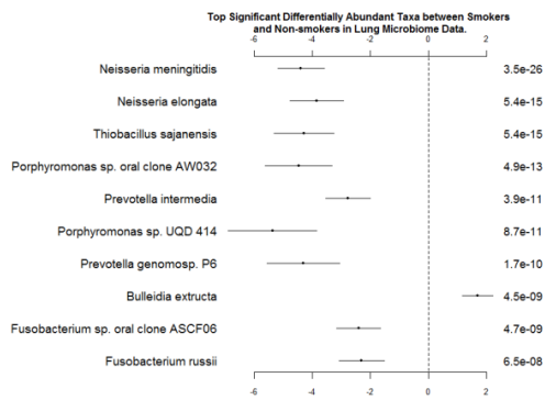
Fig. 4 - Coefficients and P-values for the Top Significant Differentially Abundant Taxa between Smokers and Nonsmokers in Lung Microbiome Data. The left column is names of taxa; the right column is p-values. The ranges of coefficients are presented in the middle column.
3.2.2. Colorectal Cancer Microbiome Data
We further applied our method to a colorectal cancer gut microbiome data originally published by Kostic et al. (2012). They studied a secondary cohort of 95 individuals with both tumor and normal tissue acquired. A more detailed description about the gut microbiome samples, collection, and protocols is available in Kostic et al. (2012). We included 274 features with zero proportion not greater than 0.8 for 185 samples in our analysis. The differential abundance analysis was to explore the association of the features between normal and tumor samples.
The original study investigated the association between Fusobacterium and colorectal carcinoma. We have listed the coefficient estimates for the significant OTUs by phylum for each genus in Figure 5. The significant differentially abundant phylum for tumor samples includes Firmicutes, Proteobacteria, Tenericutes, Actinobacteria, Bacteroidetes, and Fusobacteria. Consistent with the original study and Wang et al. (2012), Fusobacteria in cancer samples are significantly enriched. Besides, the changes in Bacteroidetes and Firmicutes phyla are similar to the original study. It is presumed in the original study that Fusobacterium species contribute to the evolvement of tumor microenvironment, leading to an altered microbiota in accordance with the ‘alpha-bug’ hypothesis introduced by Sears and Pardoll (2011). 12 of the Fusobacterium species are differentially abundant between tumor and normal samples and four of them are enriched in tumor samples, both consistent with Kostic et al. (2012).
We also include the coefficients and p-values of top significant differentially abundant species in Figure 6. Bacteroides uniformis was reported as an enriched OTUrelated species in healthy volunteers by Wang et al. (2012). Furthermore, based on the genera of the significant species, genera Lactococcus, Bacteroides, Fusobacterium, Prevotella, and Streptococcus exhibited more enriched in cancerous tissues than normal tissues, which is consistent with Gao et al. (2015). It is worth noting that two important species among the significant species in Figure 6 have been reported as antitumor bacteria. Streptococcus thermophiles has been known as an effective probiotic in deactivating risk factors of colon cancer (Wollowski, I., Rechkemmer, G., & Pool-Zobel, B. L., 2001). Ruminococcus bromii was investigated for its ability to degradation of resistant starch in the human colon to potentially prevent colon cancer (Ze, X., Duncan, S. H., Louis, P., & Flint, H. J., 2012). This confirms that ZINB is able to replicate findings from previous reports, and can be used as an efficient tool for differential abundance analysis in future microbiome studies.
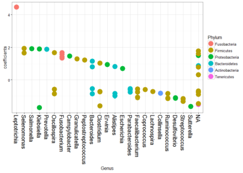
Fig. 5 - Coefficients Plot for Different Genus by Phylum in Colorectal Cancer Microbiome Data
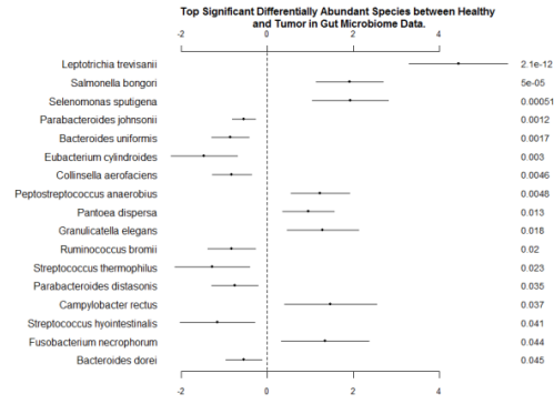
Fig. 6 - Coefficients and P-values for the Top Significant Differentially Abundant Species between Normal and Tumor Samples in Gut Microbiome Data. The left column is names of taxa; the right column is p-values. The ranges of coefficients are presented in the middle column.
4. Discussion
Existing differential abundance analysis methods in the literature can be divided into three main categories: (i) methods that address the non-negativity and over-dispersion of the microbiome counts (typically based on negative binomial distribution) typically preceded by normalization, i.e. DESeq, DESeq2, and edgeR (Anders & Huber, 2010; Li, Witten, Johnstone, & Tibshirani, 2012; Peng et al., 2015; Robinson et al., 2010; White et al., 2009), (ii) methods that rely on some transformation of the normalized counts (e.g. metagenomeSeq), and (iii) methods that handle zero-inflation by formulating some mixture model (e.g. metagenomeSeq, ZIBSeq). While most of these methods rely on some normalization scheme such as CSS, TMM, or TSS prior to modeling, the proposed method bypasses the need of normalization and accounts for sparsity and overdispersion simultaneously by directly modeling the raw counts. This makes ZINB a flexible modeling strategy, leading to interpretable differential abundance estimates in the original measurement scale. We have shown the consistency of ZINB on various types of samples in the simulation study as well as in two real human microbiome datasets.
In the lung microbiome data and some other previous studies, we have found that a common problem with the existing methods is that that they fail to consider clustered structure (if any) in the data. For example, lung microbiome data has 78 samples taken from six individuals which were treated as independent samples in the previous analyses. Therefore, a future direction of research is to incorporate random effects in the proposed ZINB model that can account for clustered structure in the observations. We have optimized our simulations to the analysis of differential abundance between two conditions of samples such as healthy versus diseased in this article. However, our method can be easily extended to more than two conditions. Finally, even though we have developed our method for microbiome data, ZINB should be applicable to other similar types of count data such as RNASeq. This strength significantly broadens the impact of ZINB among researchers in the biological community.
Список литературы
Anders, S., & Huber, W. (2010). Differential expression analysis for sequence count data. Genome Biol, 11(10), R106. doi:10.1186/gb-2010-11-10-r106
Biagi, E., Nylund, L., Candela, M., Ostan, R., Bucci, L., Pini, E., . . . De Vos, W. (2010). Through ageing, and beyond: gut microbiota and inflammatory status in seniors and centenarians. PLoS One, 5(5), e10667. doi:10.1371/journal.pone.0010667
Charlson, E. S., Bittinger, K., Haas, A. R., Fitzgerald, A. S., Frank, I., Yadav, A., . . . Collman, R. G. (2011). Topographical continuity of bacterial populations in the healthy human respiratory tract. Am J Respir Crit Care Med, 184(8), 957-963. doi:10.1164/rccm.201104-0655OC
Cho, I., & Blaser, M. J. (2012). The human microbiome: at the interface of health and disease. Nat Rev Genet, 13(4), 260-270. doi:10.1038/nrg3182
Collison, M., Hirt, R. P., Wipat, A., Nakjang, S., Sanseau, P., & Brown, J. R. (2012). Data mining the human gut microbiota for therapeutic targets. Brief Bioinform, 13(6), 751-768. doi:10.1093/bib/bbs002
De Filippo, C., Cavalieri, D., Di Paola, M., Ramazzotti, M., Poullet, J. B., Massart, S., . . . Lionetti, P. (2010). Impact of diet in shaping gut microbiota revealed by a comparative study in children from Europe and rural Africa. Proc Natl Acad Sci U S A, 107(33), 14691-14696. doi:10.1073/pnas.1005963107
Dethlefsen, L., McFall-Ngai, M., & Relman, D. A. (2007). An ecological and evolutionary perspective on human-microbe mutualism and disease. Nature, 449(7164), 811-818. doi:10.1038/nature06245
Dominguez-Bello, M. G., Costello, E. K., Contreras, M., Magris, M., Hidalgo, G., Fierer, N., & Knight, R. (2010). Delivery mode shapes the acquisition and structure of the initial microbiota across multiple body habitats in newborns. Proc Natl Acad Sci U S A, 107(26), 11971-11975. doi:10.1073/pnas.1002601107
Frank, D. N., St Amand, A. L., Feldman, R. A., Boedeker, E. C., Harpaz, N., & Pace, N. R. (2007). Molecular-phylogenetic characterization of microbial community imbalances in human inflammatory bowel diseases. Proc Natl Acad Sci U S A, 104(34), 13780-13785. doi:10.1073/pnas.0706625104
Gao, Z., Guo, B., Gao, R., Zhu, Q., & Qin, H. (2015). Microbiota disbiosis is associated with colorectal cancer. Front Microbiol, 6, 20. doi:10.3389/fmicb.2015.00020
Ghodsi, M., Liu, B., & Pop, M. (2011). DNACLUST: accurate and efficient clustering of phylogenetic marker genes. BMC Bioinformatics, 12, 271. doi:10.1186/1471-2105-12-271
Gilbert, J. A., Meyer, F., & Bailey, M. J. (2011). The future of microbial metagenomics (or is ignorance bliss?). ISME J, 5(5), 777-779. doi:10.1038/ismej.2010.178
Haddow, L. J., Mulgrew, C., Ansari, A., Miell, J., Jackson, G., Malnick, H., & Rao, G. G. (2003). Neisseria elongata endocarditis: case report and literature review. Clin Microbiol Infect, 9(5), 426-430.
Holmes, E., Li, J. V., Athanasiou, T., Ashrafian, H., & Nicholson, J. K. (2011). Understanding the role of gut microbiome-host metabolic signal disruption in health and disease. Trends Microbiol, 19(7), 349-359. doi:10.1016/j.tim.2011.05.006
Hugenholtz, P. (2002). Exploring prokaryotic diversity in the genomic era. Genome Biol, 3(2), REVIEWS0003.
Knights, D., Parfrey, L. W., Zaneveld, J., Lozupone, C., & Knight, R. (2011). Human-associated microbial signatures: examining their predictive value. Cell Host Microbe, 10(4), 292-296. doi:10.1016/j.chom.2011.09.003
Kostic, A. D., Gevers, D., Pedamallu, C. S., Michaud, M., Duke, F., Earl, A. M., . . . Meyerson, M. (2012). Genomic analysis identifies association of Fusobacterium with colorectal carcinoma. Genome Res, 22(2), 292-298. doi:10.1101/gr.126573.111
Li, J., Witten, D. M., Johnstone, I. M., & Tibshirani, R. (2012). Normalization, testing, and false discovery rate estimation for RNA-sequencing data. Biostatistics, 13(3), 523-538. doi:10.1093/biostatistics/kxr031
Mallick, H., & Tiwari, H. K. (2016). EM Adaptive LASSO-A Multilocus Modeling Strategy for Detecting SNPs Associated with Zero-inflated Count Phenotypes. Front Genet, 7, 32. doi:10.3389/fgene.2016.00032
Matsen, F. A., Kodner, R. B., & Armbrust, E. V. (2010). pplacer: linear time maximum-likelihood and Bayesian phylogenetic placement of sequences onto a fixed reference tree. BMC Bioinformatics, 11, 538. doi:10.1186/1471-2105-11-538
McMurdie, P. J., & Holmes, S. (2014). Waste not, want not: why rarefying microbiome data is inadmissible. PLoS Comput Biol, 10(4), e1003531. doi:10.1371/journal.pcbi.1003531
Nagaoka, K., Yanagihara, K., Morinaga, Y., Nakamura, S., Harada, T., Hasegawa, H., . . . Kohno, S. (2014). Prevotella intermedia induces severe bacteremic pneumococcal pneumonia in mice with upregulated platelet-activating factor receptor expression. Infect Immun, 82(2), 587-593. doi:10.1128/IAI.00943-13
Paulson, J. N., Stine, O. C., Bravo, H. C., & Pop, M. (2013). Differential abundance analysis for microbial marker-gene surveys. Nat Methods, 10(12), 1200-1202. doi:10.1038/nmeth.2658
Peng, X., Li, G., & Liu, Z. (2015). Zero-Inflated Beta Regression for Differential Abundance Analysis with Metagenomics Data. J Comput Biol. doi:10.1089/cmb.2015.0157
Robinson, M. D., McCarthy, D. J., & Smyth, G. K. (2010). edgeR: a Bioconductor package for differential expression analysis of digital gene expression data. Bioinformatics, 26(1), 139-140. doi:10.1093/bioinformatics/btp616
Robinson, M. D., & Oshlack, A. (2010). A scaling normalization method for differential expression analysis of RNA-seq data. Genome Biol, 11(3), R25. doi:10.1186/gb-2010-11-3-r25
Rogers, G. B., Carroll, M. P., Serisier, D. J., Hockey, P. M., Jones, G., & Bruce, K. D. (2004). characterization of bacterial community diversity in cystic fibrosis lung infections by use of 16s ribosomal DNA terminal restriction fragment length polymorphism profiling. J Clin Microbiol, 42(11), 5176-5183. doi:10.1128/JCM.42.11.5176-5183.2004
Samuel, B. S., & Gordon, J. I. (2006). A humanized gnotobiotic mouse model of host-archaeal-bacterial mutualism. Proc Natl Acad Sci U S A, 103(26), 10011-10016. doi:10.1073/pnas.0602187103
Sato, T., Tomida, J., Naka, T., Fujiwara, N., Hasegawa, A., Hoshikawa, Y., . . . Kawamura, Y. (2015). Porphyromonas bronchialis sp. nov. Isolated from Intraoperative Bronchial Fluids of a Patient with Non-Small Cell Lung Cancer. Tohoku J Exp Med, 237(1), 31-37. doi:10.1620/tjem.237.31
Sears, C. L., & Pardoll, D. M. (2011). Perspective: alpha-bugs, their microbial partners, and the link to colon cancer. J Infect Dis, 203(3), 306-311. doi:10.1093/jinfdis/jiq061
Segata, N., Izard, J., Waldron, L., Gevers, D., Miropolsky, L., Garrett, W. S., & Huttenhower, C. (2011). Metagenomic biomarker discovery and explanation. Genome Biol, 12(6), R60. doi:10.1186/gb-2011-12-6-r60
Sohn, M. B., Du, R., & An, L. (2015). A robust approach for identifying differentially abundant features in metagenomic samples. Bioinformatics, 31(14), 2269-2275. doi:10.1093/bioinformatics/btv165
Spor, A., Koren, O., & Ley, R. (2011). Unravelling the effects of the environment and host genotype on the gut microbiome. Nat Rev Microbiol, 9(4), 279-290. doi:10.1038/nrmicro2540
Turnbaugh, P. J., Hamady, M., Yatsunenko, T., Cantarel, B. L., Duncan, A., Ley, R. E., . . . Gordon, J. I. (2009). A core gut microbiome in obese and lean twins. Nature, 457(7228), 480-484. doi:10.1038/nature07540
Turnbaugh, P. J., Ley, R. E., Hamady, M., Fraser-Liggett, C. M., Knight, R., & Gordon, J. I. (2007). The human microbiome project. Nature, 449(7164), 804-810. doi:10.1038/nature06244
Turnbaugh, P. J., Ley, R. E., Mahowald, M. A., Magrini, V., Mardis, E. R., & Gordon, J. I. (2006). An obesity-associated gut microbiome with increased capacity for energy harvest. Nature, 444(7122), 1027-1031. doi:10.1038/nature05414
Velculescu, V. E., Zhang, L., Vogelstein, B., & Kinzler, K. W. (1995). Serial analysis of gene expression. Science, 270(5235), 484-487.
Virgin, H. W., & Todd, J. A. (2011). Metagenomics and personalized medicine. Cell, 147(1), 44-56. doi:10.1016/j.cell.2011.09.009
Wagner, B. D., Robertson, C. E., & Harris, J. K. (2011). Application of two-part statistics for comparison of sequence variant counts. PLoS One, 6(5), e20296. doi:10.1371/journal.pone.0020296
Wang, T., Cai, G., Qiu, Y., Fei, N., Zhang, M., Pang, X., . . . Zhao, L. (2012). Structural segregation of gut microbiota between colorectal cancer patients and healthy volunteers. ISME J, 6(2), 320-329. doi:10.1038/ismej.2011.109
White, J. R., Nagarajan, N., & Pop, M. (2009). Statistical methods for detecting differentially abundant features in clinical metagenomic samples. PLoS Comput Biol, 5(4), e1000352. doi:10.1371/journal.pcbi.1000352
Whitman, W. B., Coleman, D. C., & Wiebe, W. J. (1998). Prokaryotes: the unseen majority. Proc Natl Acad Sci U S A, 95(12), 6578-6583.
Winstead, J. M., McKinsey, D. S., Tasker, S., De Groote, M. A., & Baddour, L. M. (2000). Meningococcal pneumonia: characterization and review of cases seen over the past 25 years. Clin Infect Dis, 30(1), 87-94. doi:10.1086/313617
Wooley, J. C., & Ye, Y. (2009). Metagenomics: Facts and Artifacts, and Computational Challenges*. J Comput Sci Technol, 25(1), 71-81. doi:10.1007/s11390-010-9306-4
Wollowski, I., Rechkemmer, G., & Pool-Zobel, B. L. (2001). Protective role of probiotics and prebiotics in colon cancer. Am J Clin Nutr, 73(2 Suppl), 451S-455S.
Wu, G. D., Chen, J., Hoffmann, C., Bittinger, K., Chen, Y. Y., Keilbaugh, S. A., . . . Lewis, J. D. (2011). Linking long-term dietary patterns with gut microbial enterotypes. Science, 334(6052), 105-108. doi:10.1126/science.1208344
Ze, X., Duncan, S. H., Louis, P., & Flint, H. J. (2012). Ruminococcus bromii is a keystone species for the degradation of resistant starch in the human colon. ISME J, 6(8), 1535-1543. doi:10.1038/ismej.2012.4